The Universe That Humans Invented · Essay Four

The Equation on the Tombstone

Boltzmann gave physics a count. The count works. What it does not give us, by itself, is the physical event that makes completed history one-way.

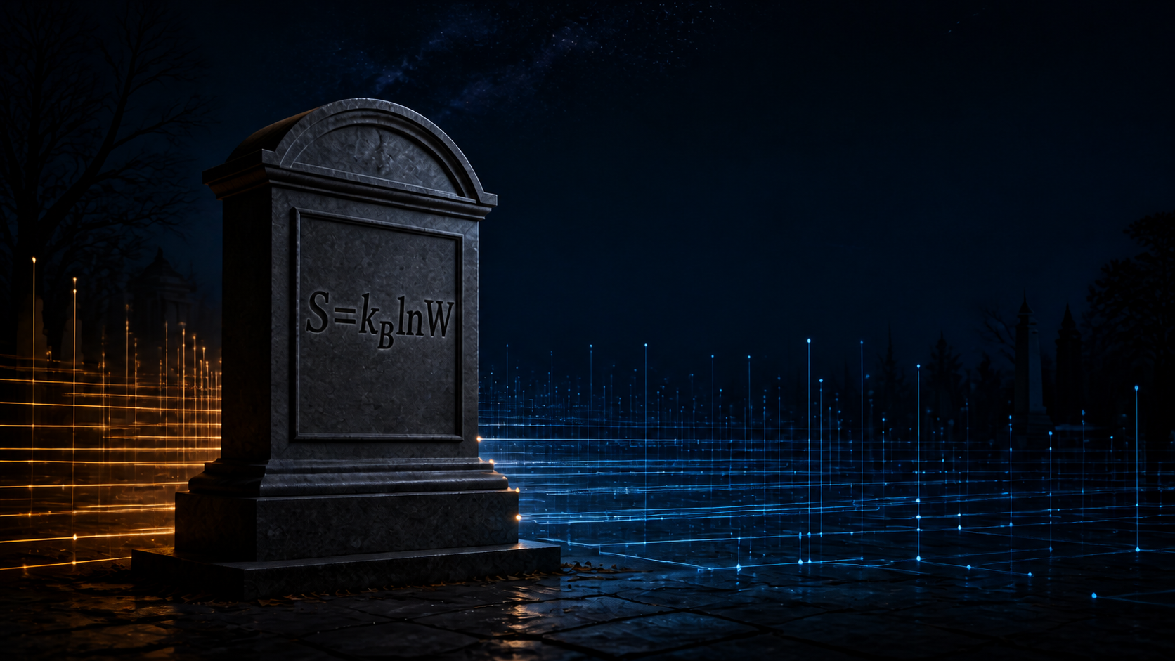
There is a grave in Vienna's Zentralfriedhof with one equation carved above Ludwig Boltzmann's bust:

It may be the most famous epitaph in science.

The formula is right. It is also routinely asked to do more than it says.

Boltzmann's 1877 work established the probabilistic relation between entropy and the multiplicity of a macrostate. Max Planck later introduced the constant $k_B$ and wrote the compact form now carved on the memorial. The equation tells us how much entropy corresponds to the number $W$ of microscopic arrangements grouped into one macroscopic description.

That is already a revolution. But it is not yet a dynamical explanation of the arrow of time.

The tombstone tells us how to count a macrostate. It does not tell us why nature writes new completed history in one direction, why the early universe occupied such a special macrostate, or why an observer's loss of access should be identified with a change in the source itself.

Those are different questions. Physics has often placed them under the same letter $S$, then celebrated the agreement of the notation as though it were an agreement of ontology.

This essay separates them.

I. Three statements that should never have been treated as one

The entropy discussion becomes much cleaner once three claims are kept apart.

The first is a state-counting statement:

Given a macrostate $M$ and a declared partition of microscopic phase space, $\mathrm{\Omega }(M)$ counts how many microstates belong to it. This is Boltzmann entropy. It says that a macrostate represented by more compatible microstates receives a larger entropy.

The second is a kinetic statement. For a dilute gas described by a one-particle distribution $f$, Boltzmann introduced a functional of the form

and, under the Boltzmann equation and its collision assumptions,

The third is the macroscopic Second Law:

These are related. They are not the same theorem.

The first defines a measure of multiplicity after a macrostate partition is chosen. The second describes a particular kinetic evolution after a factorization condition is imposed on incoming molecular pairs. The third is the observed thermodynamic arrow.

The historical confusion was not that Boltzmann's counting was wrong. It was that a conditional kinetic theorem was repeatedly advertised as though it had manufactured an irreversible law from reversible mechanics without paying for an asymmetric premise.

It had not.

II. The arrow hidden inside molecular chaos

Boltzmann's 1872 $H$-theorem uses the Stosszahlansatz, usually translated as molecular chaos. In its cleanest form, the pre-collision two-particle distribution is factorized:

For a dilute gas this is an extraordinarily productive approximation. It is one reason the Boltzmann equation works so well.

But factorization before collision is not invariant under reversing an already evolved trajectory. A collision creates correlations. Reverse all momenta after the collision and those correlations become precisely tuned incoming correlations. The reversed state remains a legal mechanical state, but it no longer satisfies the same molecular-chaos condition.

That is the arrow's entrance.

It is not an algebraic error. It is a boundary and typicality premise. The theorem proves what follows after that premise is admitted. What it cannot prove is that time-symmetric microscopic mechanics itself selected the premise.

There is a broader precision worth keeping. The mechanical and unitary quantum dynamics used in statistical mechanics are reversible under the appropriate time-reversal operation. Fundamental $T$-violation exists in the weak sector, but it is not the accepted explanation for refrigerators, gas equilibration, memory erasure, or the thermodynamic arrow. The entropy problem survives that fact.

III. Loschmidt did not refute thermodynamics. He located its missing premise

Josef Loschmidt's reversibility objection is almost offensively simple.

Take a microscopic trajectory $X(t)$ that evolves from a low-entropy macrostate toward equilibrium. Reverse every momentum at some time. The time-reversed trajectory is still admitted by the same microscopic dynamics, yet it walks back toward the low-entropy macrostate.

For every allowed entropy-increasing microscopic history, the reversible equations admit a corresponding entropy-decreasing history.

Therefore microscopic reversibility alone cannot select one member of the pair. Something else must do the selecting: a special boundary condition, a typicality measure, coarse graining, environmental coupling, a record-writing rule, or another explicitly stated source condition.

That conclusion does not make statistical mechanics unsuccessful. It makes its logical dependency visible.

Boltzmann's mature response was to make the argument statistical. Equilibrium macrostates occupy overwhelmingly larger regions of the available phase space than low-entropy macrostates. A system prepared in a low-entropy macrostate will, for typical compatible microstates, evolve toward macrostates with much larger multiplicity.

That is a powerful explanation of thermodynamic behavior. But the sentence begins with a system prepared in a low-entropy macrostate. The arrow has moved into the preparation.

IV. Zermelo found the wall at infinite time

The recurrence objection requires equally careful wording.

For a measure-preserving flow on a finite-measure phase space, Poincare recurrence says that almost every point returns arbitrarily close to its initial neighborhood, given enough time. Applied to an idealized isolated finite Hamiltonian system, that means no strictly increasing macroscopic function can remain strictly increasing forever along almost every microscopic orbit.

This does not predict that a glass of milk will visibly unmix tomorrow. It does not invalidate laboratory thermodynamics. Recurrence times for macroscopic systems can be inconceivably larger than any accessible physical timescale.

It does establish something narrower and harder: the ordinary Second Law is not an unconditional, all-times consequence of finite reversible Hamiltonian mechanics.

Zermelo did not show that entropy fails in the laboratory. He showed that the laboratory law and the microscopic recurrence theorem occupy different logical layers.

That distinction is still correct.

V. What modern physics genuinely solved, and what it did not

Modern statistical mechanics has not been idle for a century. It has built several precise answers:

• Typicality and kinetic limits explain why equilibrium behavior dominates for overwhelmingly many compatible microstates under declared preparation conditions.
• Open-system dynamics explains irreversible-looking reduced evolution when inaccessible environmental degrees of freedom are traced out.
• Quantum decoherence explains suppression of interference in a chosen pointer structure without pretending that unitary evolution itself disappeared.
• Fluctuation theorems quantify the probability of negative entropy-production fluctuations instead of banning them by decree.
• Landauer's principle ties logically irreversible erasure to a minimum thermodynamic cost of $k_{B}T\ln 2$ per bit under its physical assumptions, and the bound has been tested experimentally.
• Black-hole thermodynamics ties horizon entropy to area, forcing gravity, information, and finite capacity into the same conversation.

These are real achievements. Their equations work because their domains, reservoirs, channels, ensembles, and readout conventions are specified. That success should not be diluted.

Neither should it be inflated into a source ontology it does not provide.

The remaining question is not whether statistical mechanics predicts the behavior of a gas. It does. The remaining question is: what physical object is being counted at the source, what event makes a record complete, and what part of an entropy increase belongs to the world's ledger rather than to a laboratory quotient?

That is the question the tombstone equation leaves open.

VI. The most dangerous ambiguity in the word entropy

Physics uses several objects with the same family resemblance:

These formulas are connected by rigorous bridges in defined regimes. They should not be declared identical without naming the bridge.

Boltzmann entropy depends on a macrostate partition. Gibbs entropy depends on a probability distribution. Von Neumann entropy depends on a density operator and an algebra of observables. Thermodynamic entropy is fixed operationally through heat, work, and state variables.

The Gibbs paradox is not an unsolved scandal. Quantum indistinguishability and the correct quotient of state space resolve it. But the paradox taught a permanent lesson: the answer depends on which physical distinctions are legal. Change the state space or its quotient, and the entropy count changes.

Likewise, coarse graining is not automatically subjective whim. It may be fixed by an apparatus, an accessible algebra, a resolution scale, or a dynamical channel. But the coarse-grained description is still not the same object as the microscopic source state.

One symbol should not erase that distinction.

VII. Boltzmann's unfinished victory

Boltzmann was defending more than a formula. He was defending the physical reality of atoms when influential scientists, including Ernst Mach and Wilhelm Ostwald, regarded atomism as an unnecessary or even illegitimate hypothesis.

He was also answering Loschmidt and Zermelo from inside mechanics. Those objections were not attacks by people who failed to understand him. They were serious tests that forced the theory to state its statistical character more honestly.

Boltzmann suffered severe illness and died by suicide in 1906. It would be irresponsible to reduce that death to a morality play about scientific rejection; the historical record does not justify such a simple causal story. It is nevertheless true that he did not live to see Perrin's experiments consolidate the atomic interpretation that Einstein's Brownian-motion analysis had made quantitatively testable.

The community eventually accepted the count.

The arrow problem remained.

That is the part worth remembering. Scientific consensus can correctly adopt an equation while leaving the equation's deepest ontological question untouched.

VIII. The QTT move: stop forcing three ledgers into one number

The Artian/QTT model starts by separating four objects that standard prose often slides between:

1. Active support, $N_{\mathrm{act}}$: the finite source capacity currently available.
2. Source-created volume, $N_{\mathrm{SQ}}$: the A2 support and A3 White-Void propagation ledger, whose exact coefficient is 24.
3. Completed records, $N_{\mathrm{rec}}$: the cumulative ledger of source transactions that have actually closed.
4. Operational quotient, $N_{\mathrm{op}}$: the coarser description available through a declared laboratory access map.

A macroscopic description may shrink because many microscopic addresses become one laboratory variable. That quotient contraction does not imply that completed source records were destroyed.

This is the first hard separation:

The record ledger and the access ledger are not rival names for the same scalar. They are different coordinates with different constructors and different equality conditions.

The source coordinate is

The access coordinate uses standard quantum relative entropy. For each declared access event $e$, with state ${\rho }_e$, faithful reference ${\omega }_e$, and CPTP channel ${\mathrm{\Phi }}_e$, define

By the standard data-processing inequality,

QTT does not claim to have invented relative entropy or data processing. That mathematics belongs to Umegaki, Araki, Lindblad, Uhlmann, Petz, and the established quantum-information literature.

The QTT-specific move is to place access loss beside, but not inside, completed-record growth:

The primary object is a vector in a positive cone.

Only after the coordinates have been kept distinct does QTT form the canonical scalar total:

This is the equation that belongs beneath the equation on the tombstone.

Boltzmann counts how many microstates the laboratory groups together. The QTT equation separates what the source completed from what an access map made indistinguishable.

IX. Why the two coordinates use the same unit

Adding two non-negative quantities is easy. Justifying why they carry the same physical unit is the load-bearing step.

At one admissible QTT address, anchored modular charge is defined by

A completed A7 bundle carries

while its accessible and hidden shares satisfy

One completed record therefore has normalized charge $Q^{\mathrm{bundle}}/2\pi =1$. One unit of access loss is normalized by the same circle:

The laboratory valuation maps one normalized unit to $k_B$. Within the constructor class that permits no additional unexplained relative weight, the scalar contraction is therefore $(\mathrm{1,1})$, not $(a,b)$ with a tunable coefficient between the ledgers.

That no-extra-weight condition is essential. Without it, the master equation would acquire a new knob at exactly the point where the theory claims to remove ambiguity.

X. Where the integer 24 actually belongs

The exact integer 24 remains important. One full QTT space-quantum packet has the typed capacity decomposition

A2 assigns one such complete support packet to each Artian mass unit B = M/m_A during each source tick. It does not erase one negative record.

A3 assigns the corresponding family of twenty-four White-Void creation fronts. On the explicit branch used here, the Artian mass inventory is present together at the first counted tick and remains fixed. At tick j, the active family contains 24Bj fronts. One full SQ per active front per tick gives the finite triangular sum

This is a conditional source-volume theorem. It requires the fixed-at-origin inventory premise, the A2 packet law, the A3 active-front persistence law, and the QTT SQ volume. It is not fitted to the present cosmic volume.

If cumulative A2 support packets are separately subtracted from cumulative A3-created SQs, the result is BN_T(12N_T + 11). It equals 23B only at the first tick. It is not 23 per event, not a universal entropy coefficient, and not the source of the Second-Law sign.

The entropy arrow stands on its own typed rail: A1 orders completed events, A7 forbids undeclared deletion of their completed bundles, and standard data processing fixes the non-negative access-loss coordinate. Completed-record persistence does not borrow its sign from 24 − 1.

XI. The tombstone equation survives as a laboratory shadow

QTT does not need to destroy Boltzmann's formula. It has to explain when that formula is the correct downstream readout.

For a finite completed-event reservoir, the exact subsystem marginal is

The familiar canonical weight

appears as a controlled large-reservoir limit, with the reservoir curvature determining the approximation error. The count-to-entropy map is then isolated:

Any zero-preserving, additive, monotone map from dimensionless count entropy to laboratory entropy is linear. This fixes the role of one common scalar $k_B$. Its SI decimal remains tied to the laboratory kelvin convention.

Two premises remain visible rather than being smuggled into the conclusion: the physical local label alphabet must be finite, and the relevant microcanonical states must be equiprobable. Those are not consequences of finite capacity alone.

So the tombstone equation is not replaced. It is repositioned:

XII. A finite region cannot hide an infinite entropy bill

Once every admissible region contains a finite number of finite-capacity addresses, the local entropy bound is immediate:

and therefore

This is not a claim that QTT has regularized the same continuum local algebra more cleverly. It rejects the infinitely divisible local-address premise that produced the ultraviolet divergence in the first place.

That is an ontological replacement, not a cutoff calculation.

The distinction should be stated carefully. Finite-dimensional quantum systems, lattices, and other discrete models already have finite entropy bounds. What is QTT-specific is the claim that the finite address structure is physical source ontology rather than a computational regulator.

XIII. The quarter on a black-hole horizon

The same address budget reaches the Bekenstein-Hawking coefficient.

QTT assigns the surface-address quantum

and the completed bundle

For horizon occupancy $0\le {\eta }_H\le 1$, the completed anchor count is

Hence

and the famous quarter is

Hawking radiation is not used as the constructor of this coefficient. The effective Hawking-temperature form can be recovered later as a first-law readout after the entropy coefficient has been fixed.

This is a closed coefficient inside the QTT source ontology, not direct empirical confirmation of the microscopic address model. The bridge from the modular source unit to the full von Neumann entropy of a physical horizon remains an explicit open obligation. Without a separately declared unitary transfer channel, QTT also does not assert an evaporation trajectory or manufacture a Page curve by prose.

The exact-looking quarter is not permitted to close those different gates.

XIV. The premise-removal test

A theorem is strongest when the reader can see exactly how to break it.

The QTT entropy construction fails or changes under the following declared countermodels:

1. Remove the A2 packet law. The support count N_SQ^A2 = BN_T is no longer derived.
2. Remove persistent A3 front production. The triangular source-volume law no longer follows.
3. Remove the fixed-at-origin inventory premise. The closed form must be replaced by the exact inventory-history convolution.
4. Identify support use with negative history. The false universal 23 returns; this is a ledger-type error, not a new theorem.
5. Admit undeclared record deletion. Then the completed-record count may decrease and the record theorem fails.
6. Admit a non-CPTP access rule. Then the data-processing sign of the access term is no longer guaranteed.
7. Confuse a shrinking operational quotient with source erasure. Then an observer's compressed description is falsely counted as destruction of the completed ledger.

These are not decorative caveats. They locate the load-bearing joints.

The empirical question is correspondingly clean: does nature realize the finite source constructor that makes those premises physical? The paper closes the implication. Observation must decide whether the constructor describes the universe.

XV. What remains open

The strongest honest claim is not that entropy has been experimentally solved.

It is this:

Inside the declared finite QTT constructor class, completed-record persistence and standard access data processing form a two-coordinate positive ledger. Separately, the exact twenty-four-member A2 packet and A3 White-Void creation family produce a finite triangular source-volume ledger for a fixed-at-origin Artian mass inventory.

Several obligations remain:

• The initial ledger size is not derived. QTT reformulates the Past Hypothesis as an initial completed-record problem; it does not erase every initial-condition question.
• The finite local label alphabet and microcanonical equiprobability used in the Boltzmann reconstruction remain printed premises.
• The source-level modular charge requires an operational reconstruction protocol connecting the finite address description to independent laboratory observables.
• The horizon coefficient is closed inside the QTT constructor, while the modular-to-von-Neumann horizon bridge remains open.
• The Page-capacity envelope is conditional on a separately declared transfer channel. No transfer channel means no asserted evaporation curve.
• The source theorem has not yet been experimentally adjudicated as a unique QTT result.

That is not weakness added after the fact. It is the map of what the equations have and have not earned.

XVI. The second line on the tombstone

Boltzmann's equation should remain exactly where it is.

It tells us how many microscopic possibilities a laboratory macrostate has grouped together.

But if the QTT construction is right, it needs a second line beneath it:

The first equation counts possibilities.

The second separates completed history from lost access.

Boltzmann counted the ways a world could look the same. QTT asks what the world had to complete before those possibilities existed to be counted.

That is the proposed missing ontology of entropy.

The equation on the tombstone is not wrong.

It may be the laboratory shadow of a deeper counting ledger.

Sources and receipts

Historical and standard-physics anchors

• Ludwig Boltzmann, 1877 statistical interpretation of entropy: English translation and historical apparatus.
• H-theorem, Loschmidt objection, and Zermelo recurrence analysis: Brown and Myrvold, Studies in History and Philosophy of Modern Physics.
• Experimental Landauer bound: Berut et al., Nature 483, 187-189 (2012).
• Jacob Bekenstein, black-hole entropy: Physical Review D 7, 2333 (1973).
• Stephen Hawking, particle creation by black holes: Communications in Mathematical Physics 43, 199-220 (1975).

QTT concept anchors

• Artian's Entropy and Second-Law Reference Theorem: completed-record ledger, two-coordinate theorem, exact A2/A3 support-and-volume separation, finite entropy, horizon coefficient, and open empirical gates.
• Boltzmann Weighting from Finite Completed-Event Reservoirs: exact finite-reservoir marginal, controlled canonical limit, role of $k_B$, and explicit equiprobability obligations.
• Unified Equilibrium Law: modular-charge fifth face: the $2\pi$ bundle normalization and energy-information face.
• Black-hole information and finite address capacity: information-denial and horizon source construction without Hawking radiation as a premise.
• Quantum Traction Theory: Main Book: current source ontology, axioms, theorem dependencies, and status ledger.

Reader routes

• Quantizing and Deriving Entropy
• The Two Second Laws
• Derivation Atlas: Second Law
• Observatory: Arrow of Time
• Corpus Tree: entropy and information

Author: Ali Attar
ORCID: 0009-0008-9931-2691
Website: quantumtraction.org